Flow Matching Part 3. Paths and Schedulers

Introduction

So far our tinyflow package can only "track" probability mapping via linear function. That is, in our training algorithm for learning the (conditional) velocity field we relied on a linear map:

x_t = t * x_1 + (1 - t) x_t

In fact, the paper explains, that this specific linear map (which originates from optimal transport problem) gives us the perfect flow by minimizing the kinetic energy of the flow (see section 4.7 and references therein).

This is a fascinating topic, but without going into details, this map is a particular member of a more general class of paths called affine conditional flows or affine flows (note that we say conditional because the unconditional problem of flow matching is computationally infeasible):

x_t = alpha(t) * x_1 + sigma(t) * x_0

Affine flows and schedulers

The above formula adds two time dependent functions. The pair \(\alpha_t, \sigma_t\) is called a scheduler. Of these functions, we demand that they satisfy

alpha(0) = sigma(1) = 0
alpha(1) = sigma(0) = 1

and

In other words, as one function increases towards our ending point \(t=1\), the other decreases.

Once the affine flow is defined, we use a neural network to parametrize the velocity field.

dx_t = d_alpha(t) * x_1 + d_sigma(t) * x_0

Where d_alpha and d_sigma are derivatives of our functions (known in advance).

A note on denoising and reparametrization

In these experiments, our training setup was to train a model that represents the velocity field. From that velocity field, we obtain the flow and generate new data samples.

As an alternative, one can train a denoising model. From that model, one can then estimate velocity field by reparametrization trick (screenshot from the original paper, page 27):

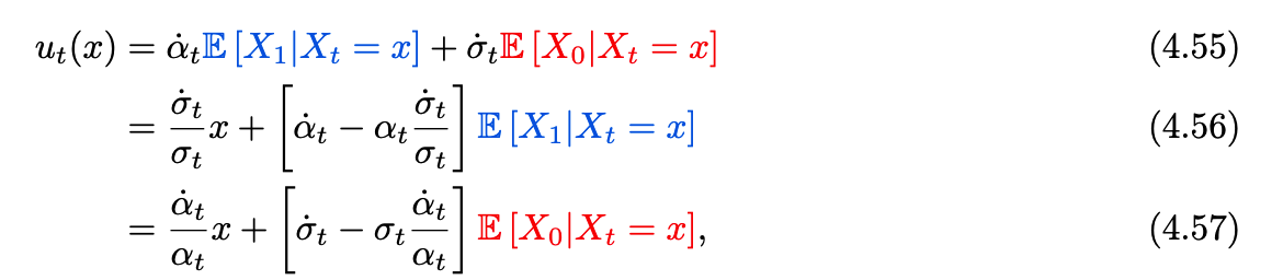
In this package I will not (at least right now) implement the reparametrization.

Possible schedulers

We can have multiple different affine paths defined by schedulers. Here are some examples:

Linear Scheduler

Linear scheduler is simply the original scheduler with which we started this project.

class LinearScheduler(BaseScheduler):
    def __init__(self):
        super().__init__()

    def alpha_t(self, t):
        return t

    def alpha_t_dot(self, t):
        return T.ones_like(t)

    def sigma_t(self, t):
        return 1 - t

    def sigma_t_dot(self, t):
        return -T.ones_like(t)

Notice the implementation of derivatives: they are required for the velocity field.

Polynomial scheduler

Another example is a polynomial scheduler:

class PolynomialScheduler(BaseScheduler):
    def __init__(self, n: int):
        super().__init__()
        self.n = n

    def alpha_t(self, t):
        return t**self.n

    def alpha_t_dot(self, t):
        return t ** (self.n - 1) * self.n

    def sigma_t(self, t):
        return 1 - t**self.n

    def sigma_t_dot(self, t):
        return -(t ** (self.n - 1)) * self.n