Implementing Flow Matching in TinyGrad.
Part 1

Posted on Fri 17 January 2025 in posts

Contents

Introduction
Flow Matching
Implementation via tinygrad
Conclusions

Introduction

In this post, I will begin a small series of implementing flow matching algorithms.

If you are not familiar with flow matching, here is a collection of papers on which I will be relying:

Flow matching guide and code is a great tutorial on various flow matching approaches. This will probably be my main reference in this project.
Flow matching for generative modeling which introduces flow matching as a modeling concept

The trick in this series of posts will be that I will try to implement everything from scratch in tinygrad. This library is very lightweight, purely pythonic and works seamlessly on Metal devices like M-series Macs.

The main implementation is done by researchers at Meta located here. We will try to rely on it as little as possible but will keep it in mind for potential comparisons. Note that I do not have CUDA GPU available, so I will be constrained in hardware.

We will start with some mathematical justifications and explanations I find useful in understanding the problem. In what follows, we assume that our data points $x$ come from a multidimensional vector space, unless otherwise specified.

Flow Matching

Flow matching is a solution to the following problem. Assume we have two distributions:

distribution $q(x)$ (which is unknown), that generates data samples (fixed in time).
distribution $p(t, x)$ which is time-dependent and at $t=0$ is a simple closed-form expression (e.g. 0-1-Gaussian) while at $t=1$ we have
$$p(1, x) \approx q(x).$$
Additionally, at any point in time $t=\tau$, we want
$$\int_{\mathcal{X}} p(\tau,x)\mathrm{d}x=1$$

Our goal is to find the "path" from $p(0, x)$ to $p(1, x)$ for each data point $x$ and $0\leq t\leq 1$. The following is a slightly wordy but, in my opinion, a non-strictly necessary introduction. We will briefly discuss concept of flows and how they help us in data generation. Finally, we will introduce the main hurdle in using flows, why flow matching is useful and how to train a flow matching model.

The problem

The difficulty of this setup is that we do not know the true path $p(t, x)$.

We cannot employ traditional approaches where a ground truth path is used to fit an approximate neural-network-based path.

Flows and Continuous Normalizing Flows

Here I will try to briefly and as simply as I can introduce flows from the point of view of dynamical systems. I highly recommend Book by Carmen Chicone and the text by Vladimir Arnold if you are interested in learning more about flows and ordinary differential equations (ODEs).

Study of dynamical systems gives us a framework of finding time-dependent functions for which we know certain information like a starting point (or initial state). Specifically, if we can solve a differential equation

$$ \begin{cases} \frac{\mathrm{d}y(t, x)}{\mathrm{d}t} = v(t, y(x)),\\ y(0) = p(x), \end{cases} $$

then the we can find the desired path. The function $v$ is called velocity vector field. From dynamical systems theory, certain conditions can be imposed on the velocity field to guarantee solution existence. These solutions are called flows: you start at one spot and the flow takes you somewhere else.

The continuous normalizing flows were defined in the Neural ordinary differential equations paper. They allow us to compute dynamics (changes) in probability via changes in the underlying random variables (samples).

Here, we are dealing with a slightly different (but not really) problem: we vary dynamics of the probability distribution directly and track the flow of the distribution from one "shape" to another. We can estimate, or model, the velocity vector field $v$ via a neural network (see the Neural ODE paper for the definition).

In a perfect scenario, each sample might come with a snap of the path that lead us to the probability distribution from which the sample originates. We would be able to train a network to estimate vector field and find an approximate flow by solving the ODE.

In an even more perfect scenario, imagine we know the true vector field $u(t,p(t, x))$.

Then we can solve the previous ODE and be able to track a path from one distribution to another seamlessly.

But therein lies the main obstacle: we do not know the true velocity vector field.

Introducing Flow Matching

Thankfully, we can still find a solution. Let's simplify the problem: instead, we look at one data point at a time.

(In fact, we can consider an aggregation over many samples but this is more complex and not computationally feasible)

Fixing a data sample $x_1$ at time $t=1$, we can define a path function which in it's simplest form can be a linear function such as:

$$X_{t} = t\,x_1 + (1-t)\,X_0.$$

Since $X_0$ comes from a known distribution, our original ODE is now solvable because we can find the true velocity field. Simply taking a derivative of $X_t$ gives us the velocity field. Such velocity field is conditional on our choice of $x_1$.

This provides us with a framework, however. For a given number of iterations, let's sample our data, train a neural network to estimate velocity field for each sample. Then at generation time, we simply solve the ODE using neural network as our velocity field and evaluate at time $t=1$.

Implementation via `tinygrad`

Now we can finally write some code.

Neural network

We need a neural network first. Our neural network needs a forward pass and we need a way to solve the ODE (following original paper and reference implementation, we call this function sample):

from tinygrad import tensor, nn

Tensor = tensor.Tensor


class MLP:
    def __init__(self, in_dim, out_dim):
        self.layer1 = nn.Linear(in_dim + 1, 64)
        self.layer2 = nn.Linear(64, 64)
        self.layer3 = nn.Linear(64, 64)
        self.layer4 = nn.Linear(64, out_dim)

    def __call__(self, x: Tensor, t: Tensor):
        # forward pass
        x = x.cat(t, dim=-1)
        x = self.layer1(x).elu()
        x = self.layer2(x).elu()
        x = self.layer3(x).elu()
        return self.layer4(x)

    def sample(self, x: Tensor, t: Tensor, h_step):
        # this is where the ODE is solved
        # d/dt x_t = u_t(x_t|x_1)
        # explicit midpoint method https://en.wikipedia.org/wiki/Midpoint_method
        t = t.reshape((1, 1))
        t = t.repeat(x.shape[0], 1)
        x_t_next = x + h_step * self(x + h_step / 2 * self(x, t), t + h_step / 2)

        return x_t_next

Training algorithm

Our training is done by sampling random snapshots of the flow at various times and minimizing the loss function. Choose mean squared error between the neural network and the chosen (conditional) path function.

from tinygrad.nn.optim import AdamW
from tinygrad.nn.state import get_parameters
from tinygrad.tensor import Tensor as T
from tqdm.auto import tqdm


num_iter = 10000

model = MLP(2, 2)
optim = AdamW(get_parameters(model), lr=0.01)
T.training = True
for iter in tqdm(range(num_iter)):
    # dataset used in the reference implementation
    x = make_moons(256, noise=0.05)[0]
    # end state, data we would like to arrive at from noise

    x_1 = T(x.astype("float32"))  # pyright: ignore
    x_0 = T.randn(*x_1.shape)  # start state, data we get from pure noise
    t = T.randn(x_1.shape[0], 1)  # time grid

    # linear path from noise to data;
    # noise at t=0, data at t=1
    # see equation 2.5 in https://arxiv.org/pdf/2412.06264
    x_t = t * x_1 + (1 - t) * x_0
    dx_t = x_1 - x_0  # see eq 2.9 on page 6 of https://arxiv.org/pdf/2412.06264
    # parametric velocity field u^theta_t(x)
    out = model(x_t, t)
    optim.zero_grad()

    loss = T.mean((out - dx_t) ** 2)  # pyright: ignore
    if iter % 50 == 0:
        print(f"Loss: {loss.item()}")
    # the reason loss has dx_t is because this is the simplest implementation of flow:
    # technically loss is MSE(out, u_t(x_t|x_1))
    # where u_t(x|x_1) is d/dt(x_t)==d/dt(t*x_1 + (1-t)*x_0)
    loss.backward()
    optim.step()

Evaluation

Finally, we are ready to compute flow from a random noise to the actual dataset (moons). The snippet is below.

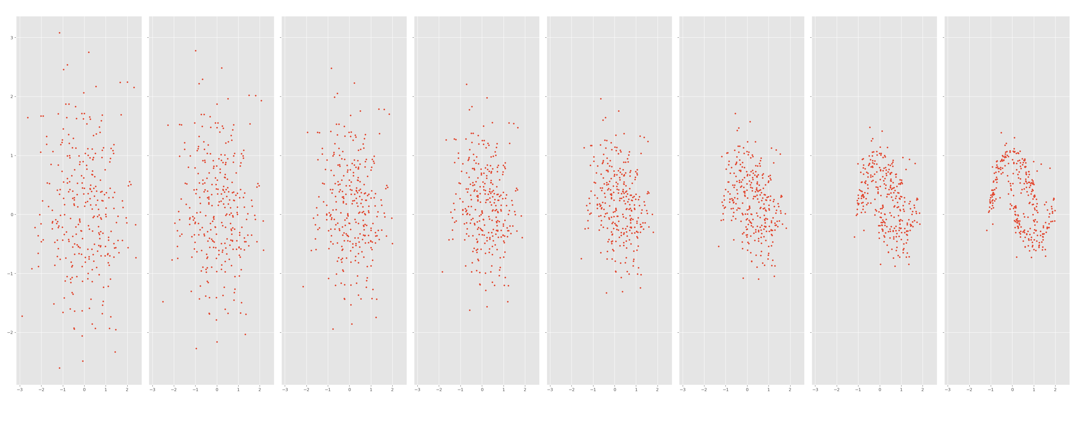
# after training, we sample
x = T.randn(300, 2)
h_step = float(1 / 8)
fig, ax = plt.subplots(1, int(1 / h_step), figsize=(30, 4), sharex=True, sharey=True)
time_grid = T.linspace(0, 1, int(1 / h_step))

i = 0
for t in time_grid:
    ax[i].scatter(x.numpy()[:, 0], x.numpy()[:, 1], s=10, c="blue")
    x = model.sample(x, t, h_step)
    i += 1
plt.tight_layout()
plt.show()

The result

We can see in the figure below how the process of flow matching is starting from random noise and moves to our moon dataset. Each figure represents a snapshot in time.

Flow matching from noise to moons

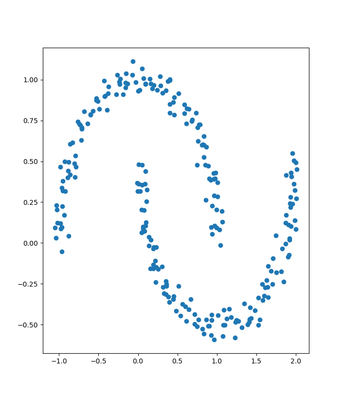
Compare the result above to the true moon dataset below

True dataset

Conclusions

Following the reference implementations and the original papers, we went through the end-to-end implementation of the most basic flow matching. Since by itself the problem can be very hard to solve, we simplified it to find the path conditionally. We create a linear path from a given example and train a neural network on snapshots of this linear path.

Finally, we are in the position to actually solve the ODE and generate new examples from noise based on the dataset used in training.

One technical challenge is that we used tinygrad library instead of pytorch to write the solution. I like using tinygrad for such small projects because it's a great opportunity to both learn the library and learn the algorithm.

This was an introductory example with a simple path and a simple solver. In following posts, I would like to discuss adding more advanced ODE solvers, other flow algorithms and potentially any optimizations we can do. One thing I would like to try on the hardware I have is to train image generation models.